监督学习

1. 线性回归

梯度下降一元线性回归

import numpy as np
import matplotlib.pyplot as plt

# 载入数据
data = np.genfromtxt("data.csv", delimiter=",")
x_data = data[:,0]
y_data = data[:,1]

# 学习率learning rate
lr = 0.0001
# 截距
b = 0 
# 斜率
k = 0 
# 最大迭代次数
epochs = 50

# 最小二乘法
def compute_error(b, k, x_data, y_data):
    totalError = 0
    for i in range(0, len(x_data)):
        totalError += (y_data[i] - (k * x_data[i] + b)) ** 2
    return totalError / float(len(x_data)) / 2.0

def gradient_descent_runner(x_data, y_data, b, k, lr, epochs):
    # 计算总数据量
    m = float(len(x_data))
    # 循环epochs次
    for i in range(epochs):
        b_grad = 0
        k_grad = 0
        # 计算梯度的总和再求平均
        for j in range(0, len(x_data)):
            b_grad += (1/m) * (((k * x_data[j]) + b) - y_data[j])
            k_grad += (1/m) * x_data[j] * (((k * x_data[j]) + b) - y_data[j])
        # 更新b和k
        b = b - (lr * b_grad)
        k = k - (lr * k_grad)
    return b, k

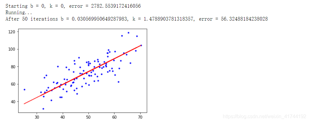
print("Starting b = {0}, k = {1}, error = {2}".format(b, k, compute_error(b, k, x_data, y_data)))
print("Running...")
b, k = gradient_descent_runner(x_data, y_data, b, k, lr, epochs)
print("After {0} iterations b = {1}, k = {2}, error = {3}".format(epochs, b, k, compute_error(b, k, x_data, y_data)))

#画图
plt.plot(x_data, y_data, 'b.')
plt.plot(x_data, k*x_data + b, 'r')
plt.show()

梯度下降法-多元线性回归

import numpy as np
from numpy import genfromtxt
import matplotlib.pyplot as plt  
from mpl_toolkits.mplot3d import Axes3D  

# 读入数据 
data = genfromtxt(r"Delivery.csv",delimiter=',')

# 切分数据
x_data = data[:,:-1]
y_data = data[:,-1]

# 学习率learning rate
lr = 0.0001
# 参数
theta0 = 0
theta1 = 0
theta2 = 0
# 最大迭代次数
epochs = 1000

# 最小二乘法
def compute_error(theta0, theta1, theta2, x_data, y_data):
    totalError = 0
    for i in range(0, len(x_data)):
        totalError += (y_data[i] - (theta1 * x_data[i,0] + theta2*x_data[i,1] + theta0)) ** 2
    return totalError / float(len(x_data))

def gradient_descent_runner(x_data, y_data, theta0, theta1, theta2, lr, epochs):
    # 计算总数据量
    m = float(len(x_data))
    # 循环epochs次
    for i in range(epochs):
        theta0_grad = 0
        theta1_grad = 0
        theta2_grad = 0
        # 计算梯度的总和再求平均
        for j in range(0, len(x_data)):
            theta0_grad += (1/m) * ((theta1 * x_data[j,0] + theta2*x_data[j,1] + theta0) - y_data[j])
            theta1_grad += (1/m) * x_data[j,0] * ((theta1 * x_data[j,0] + theta2*x_data[j,1] + theta0) - y_data[j])
            theta2_grad += (1/m) * x_data[j,1] * ((theta1 * x_data[j,0] + theta2*x_data[j,1] + theta0) - y_data[j])
        # 更新b和k
        theta0 = theta0 - (lr*theta0_grad)
        theta1 = theta1 - (lr*theta1_grad)
        theta2 = theta2 - (lr*theta2_grad)
    return theta0, theta1, theta2

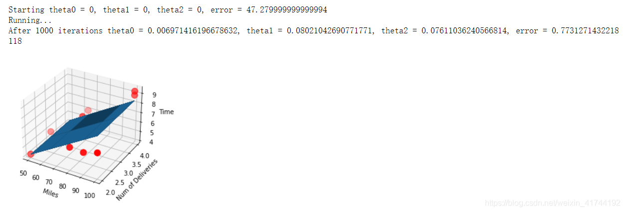
print("Starting theta0 = {0}, theta1 = {1}, theta2 = {2}, error = {3}".
      format(theta0, theta1, theta2, compute_error(theta0, theta1, theta2, x_data, y_data)))
print("Running...")
theta0, theta1, theta2 = gradient_descent_runner(x_data, y_data, theta0, theta1, theta2, lr, epochs)
print("After {0} iterations theta0 = {1}, theta1 = {2}, theta2 = {3}, error = {4}".
      format(epochs, theta0, theta1, theta2, compute_error(theta0, theta1, theta2, x_data, y_data)))

ax = plt.figure().add_subplot(111, projection = '3d') 
ax.scatter(x_data[:,0], x_data[:,1], y_data, c = 'r', marker = 'o', s = 100) #点为红色三角形  
x0 = x_data[:,0]
x1 = x_data[:,1]
# 生成网格矩阵
x0, x1 = np.meshgrid(x0, x1)
z = theta0 + x0*theta1 + x1*theta2
# 画3D图
ax.plot_surface(x0, x1, z)
#设置坐标轴  
ax.set_xlabel('Miles')  
ax.set_ylabel('Num of Deliveries')  
ax.set_zlabel('Time')  
  
#显示图像  
plt.show()  

2. 逻辑回归

逻辑回归原理与推导
梯度下降法-逻辑回归

import matplotlib.pyplot as plt
import numpy as np
from sklearn.metrics import classification_report
from sklearn import preprocessing
# 数据是否需要标准化
scale = True

# 载入数据
data = np.genfromtxt("LR-testSet.csv", delimiter=",")
x_data = data[:,:-1]
y_data = data[:,-1]
    
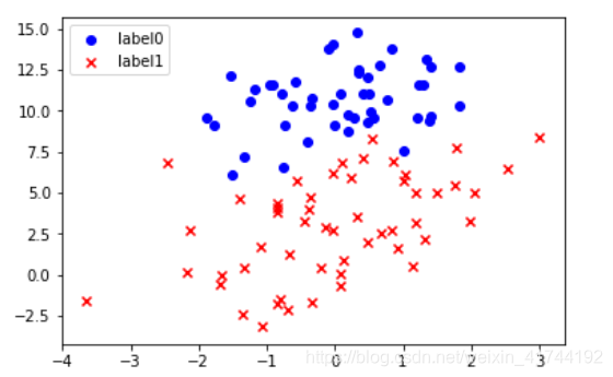
def plot():
    x0 = []
    x1 = []
    y0 = []
    y1 = []
    # 切分不同类别的数据
    for i in range(len(x_data)):
        if y_data[i]==0:
            x0.append(x_data[i,0])
            y0.append(x_data[i,1])
        else:
            x1.append(x_data[i,0])
            y1.append(x_data[i,1])

    # 画图
    scatter0 = plt.scatter(x0, y0, c='b', marker='o')
    scatter1 = plt.scatter(x1, y1, c='r', marker='x')
    #画图例
    plt.legend(handles=[scatter0,scatter1],labels=['label0','label1'],loc='best')
    
plot()
#查看数据
plt.show()

# 数据处理，添加偏置项
x_data = data[:,:-1]
y_data = data[:,-1,np.newaxis]

print(np.mat(x_data).shape)
print(np.mat(y_data).shape)
# 给样本添加偏置项
X_data = np.concatenate((np.ones((100,1)),x_data),axis=1)

def sigmoid(x):
    return 1.0/(1+np.exp(-x))

def cost(xMat, yMat, ws):
    left = np.multiply(yMat, np.log(sigmoid(xMat*ws)))
    right = np.multiply(1 - yMat, np.log(1 - sigmoid(xMat*ws)))
    return np.sum(left + right) / -(len(xMat))

def gradAscent(xArr, yArr):
    
    if scale == True:
        xArr = preprocessing.scale(xArr)
    xMat = np.mat(xArr)
    yMat = np.mat(yArr)
    
    lr = 0.001
    epochs = 10000
    costList = []
    # 计算数据行列数
    # 行代表数据个数，列代表权值个数
    m,n = np.shape(xMat)
    # 初始化权值
    ws = np.mat(np.ones((n,1)))
    
    for i in range(epochs+1):             
        # xMat和weights矩阵相乘
        h = sigmoid(xMat*ws)   
        # 计算误差
        ws_grad = xMat.T*(h - yMat)/m
        ws = ws - lr*ws_grad 
        
        if i % 50 == 0:
            costList.append(cost(xMat,yMat,ws))
    return ws,costList

# 训练模型，得到权值和cost值的变化
ws,costList = gradAscent(X_data, y_data)
print(ws)

if scale == False:
    # 画图决策边界
    plot()
    x_test = [[-4],[3]]
    y_test = (-ws[0] - x_test*ws[1])/ws[2]
    plt.plot(x_test, y_test, 'k')
    plt.show()

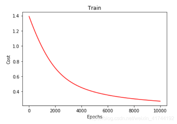
# 画图 loss值的变化
x = np.linspace(0,10000,201)
plt.plot(x, costList, c='r')
plt.title('Train')
plt.xlabel('Epochs')
plt.ylabel('Cost')
plt.show()

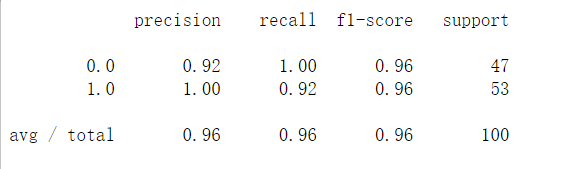
# 预测
def predict(x_data, ws):
    if scale == True:
        x_data = preprocessing.scale(x_data)
    xMat = np.mat(x_data)
    ws = np.mat(ws)
    return [1 if x >= 0.5 else 0 for x in sigmoid(xMat*ws)]

predictions = predict(X_data, ws)

print(classification_report(y_data, predictions))

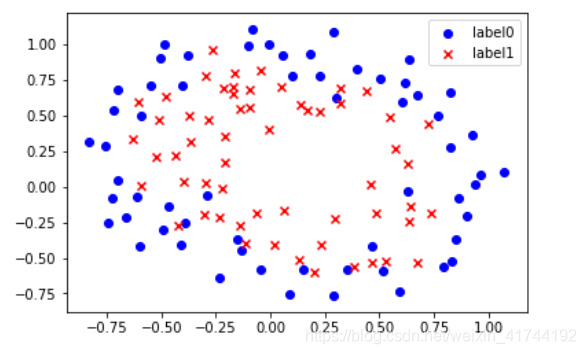
梯度下降法-非线性逻辑回归

import matplotlib.pyplot as plt
import numpy as np
from sklearn.metrics import classification_report
from sklearn import preprocessing
from sklearn.preprocessing import PolynomialFeatures
# 数据是否需要标准化
scale = False

# 载入数据
data = np.genfromtxt("LR-testSet2.txt", delimiter=",")
x_data = data[:,:-1]
y_data = data[:,-1,np.newaxis]
    
def plot():
    x0 = []
    x1 = []
    y0 = []
    y1 = []
    # 切分不同类别的数据
    for i in range(len(x_data)):
        if y_data[i]==0:
            x0.append(x_data[i,0])
            y0.append(x_data[i,1])
        else:
            x1.append(x_data[i,0])
            y1.append(x_data[i,1])

    # 画图
    scatter0 = plt.scatter(x0, y0, c='b', marker='o')
    scatter1 = plt.scatter(x1, y1, c='r', marker='x')
    #画图例
    plt.legend(handles=[scatter0,scatter1],labels=['label0','label1'],loc='best')
    
plot()
plt.show()

# 定义多项式回归,degree的值可以调节多项式的特征
poly_reg  = PolynomialFeatures(degree=3) 
# 特征处理
x_poly = poly_reg.fit_transform(x_data)

def sigmoid(x):
    return 1.0/(1+np.exp(-x))

def cost(xMat, yMat, ws):
    left = np.multiply(yMat, np.log(sigmoid(xMat*ws)))
    right = np.multiply(1 - yMat, np.log(1 - sigmoid(xMat*ws)))
    return np.sum(left + right) / -(len(xMat))

def gradAscent(xArr, yArr):
    
    if scale == True:
        xArr = preprocessing.scale(xArr)
    xMat = np.mat(xArr)
    yMat = np.mat(yArr)
    
    lr = 0.03
    epochs = 50000
    costList = []
    # 计算数据列数，有几列就有几个权值
    m,n = np.shape(xMat)
    # 初始化权值
    ws = np.mat(np.ones((n,1)))
    
    for i in range(epochs+1):             
        # xMat和weights矩阵相乘
        h = sigmoid(xMat*ws)   
        # 计算误差
        ws_grad = xMat.T*(h - yMat)/m
        ws = ws - lr*ws_grad 
        
        if i % 50 == 0:
            costList.append(cost(xMat,yMat,ws))
    return ws,costList

# 训练模型，得到权值和cost值的变化
ws,costList = gradAscent(x_poly, y_data)
print(ws)


# 获取数据值所在的范围
x_min, x_max = x_data[:, 0].min() - 1, x_data[:, 0].max() + 1
y_min, y_max = x_data[: